THE MODAL ANALYSIS OF AN EXTENDABLE/RETRACTABLE CANTILEVERED TRI-SECTIONED BEAM WITH VARIOUS END STIFFNESS CONFIGURATIONS
By
Trevor Douglas Roebuck
Bachelor of Science
-------------------------------------------------------------------
Submitted in Partial Fulfillment of the
Requirements for the Degree of Master of Science in the
Department of Mechanical Engineering
2005
-------------------------------------------- -- -----------------------------------------------
Department of Mechanical Engineering Department of Mechanical Engineering
Director of Thesis 2nd Reader
-----------------------------------
Dean of the
Abstract
This research exposes vibration characteristics of a retractable/extendable tri-sectioned cantilevered beam with overlapping segments and variable end mount stiffness by methods of dynamic testing and Finite Element Analysis. In addition, affects due to bulkhead arrangements are tested, modeled, and classified in order of the first two resonant frequencies. By comparison, of the Finite Element Analysis data to actual testing data the natural resonant frequency trends are confidently predicted. Using the same Finite Element Analysis model, two specialized bulkheads are created and proven to increase the natural resonant frequency characteristics throughout any of the beams various methods of retraction/extension. This achieves the goal of forcing the beams resonant frequencies higher, permitting the tri-segmented beam to mount to low resonant frequency structures without threat of the failures caused by vibration.
TABLE OF CONTENTS
Abstract........................................................................................................................ 2
List of Tables.............................................................................................................. 5
List of Figures............................................................................................................ 6
Introduction.............................................................................................................. 8
General Information.......................................................................................................................................... 8
Problem Definition............................................................................................................................................... 9
Research Objectives.......................................................................................................................................... 10
Roadmap.................................................................................................................................................................. 11
Theory.......................................................................................................................... 13
Research..................................................................................................................... 19
Equipment............................................................................................................................................................... 19
Test Specimen...................................................................................................................................................... 19
Test Equipment................................................................................................................................................... 25
Data Acquisition................................................................................................................................................ 26
Accelerometers.................................................................................................................................................. 26
Signal Processing System.................................................................................................................................. 27
Manipulation...................................................................................................................................................... 29
Testing..................................................................................................................................................................... 30
Main Fixture....................................................................................................................................................... 30
SRS/Spacing...................................................................................................................................................... 30
HSS/Spacing..................................................................................................................................................... 34
LSS/Spacing...................................................................................................................................................... 35
Intermediate Joint Arrangements.................................................................................................................... 37
Joint 1-2............................................................................................................................................................. 37
Joint 2-3............................................................................................................................................................. 38
Extension/Retraction......................................................................................................................................... 39
Extending Beam Three 1st.................................................................................................................................. 39
Equally Extending Beams.................................................................................................................................. 40
Extending Beam One 1st.................................................................................................................................... 41
Results and Discussion...................................................................................... 41
Main Fixture Spacing........................................................................................................................................ 48
Intermediate Joint Arrangements............................................................................................................. 50
Joint 1-2............................................................................................................................................................... 51
Joint 2-3............................................................................................................................................................... 54
Original Retraction/Extension Tests...................................................................................................... 57
Extending Beam 3 First..................................................................................................................................... 58
Equally Extending............................................................................................................................................. 61
Extending Beam 1 First..................................................................................................................................... 63
Beam Adaptation.................................................................................................... 66
Adapted Retraction/Extension Tests....................................................................................................... 67
Extending Beam 3 First..................................................................................................................................... 67
Equally Extending............................................................................................................................................. 69
Extending Beam 1 First..................................................................................................................................... 70
Summary of Results............................................................................................. 71
Conclusion................................................................................................................ 73
Areas of improvement and possible future testing........................ 74
List of Tables
Table 1: Data
Acquisition System configuration
Table
2: Beam 1 mounting pad and accelerometer
location.
Table
3: Beam 2 mounting pad and accelerometer
location.
Table
4: Beam 3 mounting pad and accelerometer
location.
Table
5: Test name of fixture spacer selection
at 24 inch Main fixture spacing.
Table
6: Test name of fixture spacer selection
at 18 inch Main fixture spacing.
Table
7: Test name of fixture spacer selection
at 12 inch Main fixture spacing.
Table
8: Test name and bulkhead location.
Table
9: Test name and bulkhead location.
Table
10: Mass applied and respective
deflection.
List of Figures
Figure
1: Forced oscillating system with a
single degree of freedom.
Figure
2: Unforced oscillating system with a
single degree of freedom.
Figure
3: Unforced oscillating system with 3 degrees
of freedom.
Figure
4: Vacuum wrapping of the 2nd
beam’s two halves.
Figure
5: Two cured halves of the 2nd
beam.
Figure
6: Intermediate joint between the 2nd and 3rd beam.
Figure
7: 3rd beam internal
bulkheads.
Figure
8: CATIA 3-D drawing of the mounting jig
assembly.
Figure
9: Closer look at the inner collar of
the mounting jig assembly.
Figure
10: Completely assembled beam mounted to
the MTS shaker table.
Figure
12- PCB 353B03 accelerometer.
Figure
14: Resonant frequency scan at fully
extended.
Figure
15: Fully extended beam mounted to the
MTS shaker table.
Figure
16: 1st resonant mode FEA
model.
Figure
17: 2nd resonant mode FEA
model.
Figure
18: 3rd resonant mode FEA model.
Figure
19: 1st Resonant Frequency
vs. Main Fixture Spacing
Figure
20: 2nd Resonant Frequency
vs. Main Fixture Spacing
Figure
21: FEA and Model Comparison
Figure
22: 1st Resonant Frequency
vs. Bulkhead Position
Figure
23: 2nd Resonant Frequency
vs. Bulkhead Position
Figure
24: Bulkhead position model comparison
Figure
25: 1st resonant frequency of
2nd beam bulkhead position.
Figure
26: 2nd resonant frequency of
2nd beam bulkhead position.
Figure
27: 2nd beam model comparison
of bulkhead position
Figure
28: Resonant frequency vs. Extension
from beam 3-1
Figure
29: FEA and model comparison vs. length
Figure
30: Resonant frequency vs. Equal
Extension of Beams
Figure
31: Resonant Frequency vs. Beam
Extension 1-3
Figure
32: FEA and Model Comparison vs. Length
Figure
33: Adapted beam resonant frequency vs.
length (extending 3-1)
Figure
34: Adapted beam resonant frequency vs.
length (extending equally)
Figure
35: Adapted beam resonant frequency vs.
length (extending 1-3)
Figure
36: Amplitude vs. Frequency (with noise)
Introduction
General
Information
Gulfstream, a General Dynamic
Company founded in 1958, has been steadily working on improving the quality of
flight. In both February of 1998 and
2004, Gulfstream was awarded the highest honor in
The current full-scale elongated
nose is roughly 45 feet in length. With
the elongated nose in place, the FAA is prohibiting the aircraft from taking
off and landing at public airports. Gulfstream is attempting to resolve this
particular problem by making the elongated nose extendable and
retractable. This opens a new area for
study in vibration analysis within multi segmented cantilevered beams thus creating
the partnership between
Problem Definition
This researches main purpose is to provide a resonant frequency key of actual tested data for comparison and validation of Gulfstream’s Finite Element Analysis (GS-FEA). This will provide the necessary information in order to redesign or adapt the extendable/retractable beam such that the beam’s resonant frequencies will not be not be similar to the planes. Resonant frequencies nearing the plane’s resonant frequency could cause the cantilevered structure to fail.
Even with the help of the
University’s vibration testing facility, the full-scale model is unable to be
tested. Instead, Gulfstream constructed
a quarter scale model of the retractable/extendable tri-cantilevered system. This is done to ensure accurate GS-FEA test
results. By testing the quarter scale
model for various end stiffness and comparing the results to the quarter scale GS-FEA
results a level of confidence is established.
Early meetings introduced the importance of understanding the resonant
signatures throughout retraction/extension of the system along with the
different possibilities of retraction/extension. With the ability to test and understand these
resonant frequencies an even more reliable comparison can be made between the
actual and the GS-FEA quarter scale model.
Due to the complexity of the systems overlapping segments, inter segment
and endpoint stiffness the vibration results were less intuitive than
originally expected and testing methods needed to be revised accordingly. Originally, for rough early predictions, the
quarter scale model was treated as a simple cantilevered, but upon testing, the
system’s measured resonant frequencies were not as expected. This over simplification led to the
introduction of more difficult calculations and the addition of an on
Research Objectives
The main purpose of this research is to confidently locate and provide the non-homogeneous, overlapping multi-segmented structure’s resonant frequencies for various conditions. In order to provide the information three separate types of tests consisting of subtests must be conducted and go as follows:
I. Main Fixture Tests
A). Solid Round Aluminum Spacers
1). 12 inch Main Bulkhead Spacing
2). 18 inch Main Bulkhead Spacing
3). 24 inch Main Bulkhead Spacing
B). Heavy Spring Spacers
C). Light Spring Spacers
II. Intermediate Joint Arrangements Tests
A). Joint 1-2
B). Joint 2-3
III. Extension/Retraction Tests
A). Extension of Beam Three 1st
B). Equal Extension of the Beams
C). Extension of
Beam One 1st
Once all of the tests were completed a finite element analysis model, comparable to the one used by Gulfstream, was used to validate and establish a level of confidence in the results.
Roadmap
For any research to serve a purpose
it must be understandable, concise and reproducible. This allows the research to be used as a stepping
stone for future researchers. When
beginning this research there was plenty information and studies found on the
vibration of cantilevered objects. There
even exists vibration research on non-homogeneous multi-segmented structures
with dissimilar cross-sectional areas.
These types of studies were readily found in Civil Engineering while
researching vibrations in buildings and free standing structures, but there
were not many stepping stones available for non-homogenous structures with
overlapping sections. The list of
available resources narrowed even more when looking at the vibration signatures
during retraction or extension of non-homogeneous, multi-segmented structures
with dissimilar cross-sectional areas and overlapping segments. Although the predecessor to this research was
the closest research found on non-homogeneous structures with overlapping
segments, it too never covered the changes in resonant frequencies during
retraction/extension [13]. What this research
did was selected and acquired the proper recording instruments such as the data
acquisition system, accelerometers and data collection programs. It also provided a method to operating the
Material Test Systems (MTS) shaker table and established a process of running
tests that scanned the correct range of frequencies. The previous research tested the influence of
end-mount flexibility on the resonant frequency response of a non-homogeneous
structure with overlapping segments and dissimilar cross-sectional areas. This research gave workable results
comparable to those witnessed at Gulfstream on their finite element analysis
program. This provided the ground work
for the current research and gave validity to the program setup between
Gulfstream and the
The current research begins where the previous research The Modal Analysis of a Cantilevered Tri-Sectioned Beam with Various End Stiffness Configurations leaves off. Where that research stops at the variety of three different end-mount configurations, ranging from solid round aluminum spacers (SRAS), light spring spacers (LSS), and heavy spring spacers (HSS), the current research consists of nine different end-mount configurations. These new tests include the previously selected three spacers and added the variable of three main fixture bulkhead locations. In addition to these advancements, this research also examines the changes in resonant frequencies due to rearranging the internal bulkheads within the end of each of the two larger beams and the influence retracting and extending has on resonant frequencies. This is done through the use of actual quarter scale vibration testing and finite element analysis modeling. This research also makes suggestions for improvement of the beams and future research work.
Theory
Structures containing supported mass such as in cantilevered systems are cause to experience resonant frequencies. The resonant frequencies are frequencies at which a system, if displaced from rest, tends to oscillate at a frequency that is dependant upon the mass and restoring force stiffness. In addition, resonant frequencies are frequencies where the amplitude increases when in contact with a forcing function with the same frequency. Increased amplitudes can lead to large displacements and are catastrophic by resulting in large stresses. For this exact case, it is important to study the natural resonant frequency of Gulfstream’s multi-segmented cantilevered structure, because the plane itself will act as a forcing function. Given that the plane’s natural frequency is low, it is imperative to force the cantilevered structure’s resonant frequencies higher. This is done by increasing the stiffness or by decreasing the mass, but first the natural resonant frequencies are found. The basic equation of motion with a forcing function F(t) for a single concentrated point mass (m) located at the center of mass with a known stiffness (k) is given by the following:
![]() Equation
1
Equation
1
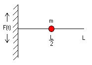
Figure 1: Forced oscillating system with a
single degree of freedom.
Equation 1 is useful for obtaining system responses to any particular forcing function. For the purpose of this research the objective is to establish the resonant frequencies for various joint, length and endpoint conditions and this is done by setting F(t) equal to zero reducing equation 1. For a basic single point mass concentration (m) located at its center of mass and stiffness (k) the resonant frequency can be found by solving following equation of motion:
![]() Equation
2
Equation
2
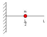
Figure 2: Unforced oscillating system with
a single degree of freedom.
Assuming all of the mass is concentrated at a single point will give poor results for the triple cantilevered beam system being studied, because this yields results comparable to a standard rigidly fixed cantilevered beam where the frequencies increase to infinity as it retracts. A method needs to be used such that the main fixture’s stiffness k is represented along with the stiffness due to all three beams, and both beam joint stiffness. All of the mass must be accounted for relative to its respective stiffness. For the case using solid round aluminum spacers (SRAS) the fixture is assumed to be an end mount of infinite stiffness and k will remain the stiffness coefficient for the beam, but for the stiff and light springs more intricate details must included about the end mount stiffness. The cases involving the light and stiff springs require experimental results to reveal the end mount stiffness. Equation 1 is used in a system with a single degree of freedom. This equation works well for simple systems, but would be hard to adapt to account for overlapping segments or beams that retract inside into each other. Using this equation would be an oversimplification of this system. Although this equation of motion, for a simple system, is inadequate for this triple segmented beam system, it can be added to in order to increase accuracy. By increasing the degrees of freedom or the number of coordinates used to describe the systems motion more details pertaining to the system can be incorporated. More details brought into the model increases the chances of the equations of motion accurately modeling the complexity greatly increase. This is done by expanding the equation of motion into a matrix where each mass concentration is fixed by stiffness relative to its neighboring mass concentrations. An example of a three mass system:
 Equation
3
Equation
3
These equations of motions are enough to represent each individual beam with a single point mass concentration located at the center of mass of each beam.
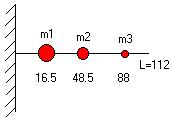
Figure 3: Unforced oscillating system with
3 degrees of freedom.
These equations of motion include more detail about the system, but require additional information for k1 since it needs to incorporate the stiffness coefficient for the main fixture.
For dependable frequency results of a cantilevered beam with three segments capable of being retracted into each other the equations of motions become more difficult to solve. These equations become difficult, because the masses and stiffness vary and for special areas are not continuous. In order to keep track of these discontinuities step functions are required and involve computer programming. For a standard cantilevered beam where L is the length of the beam, E is Young’s modulus and I is the moment of inertia of the beam the stiffness k is found by the following equation:
![]() Equation
4
Equation
4
For a system that retracts into itself there exists a period within its end joint bulkhead area where the beams stiffness increases, when a mass concentration passes through this region it acts as a mass concentration of the previous beam and needs to be represented by step functions. The concentration of this research is to ensure an accurate frequency profile of various endpoint conditions, joint stiffness, and lengths for model verification. This process is tedious and not necessary for the success of this research, instead a simplified third method of model verification is done. Although a possibility for future research, rough calculations are done by use of Dunkerley’s equation:
![]() Equation
5
Equation
5
Equation 6 is commonly used for dynamically testing structures where w11 is the resonant frequency of a structure, w22 is the resonant frequency of an additional test mass, and w1 is the total resonant frequency of the structure and the test mass combined. The test mass must make up a large percentage of the total mass in order to make noticeable changes in resonant frequencies. For simplification of calculations and this researches purpose the second and third beam are considered to be test masses and for the purpose it is used here it is considered to be sufficiently large. This is done since it is less difficult to calculate the resonant frequency of each beam individually and then add them together. By use of Dunkerley’s equation and a similar equation used in electronics for equivalent resistance of resisters running in a parallel circuit Dunkerley’s equation becomes:
![]() Equation
6
Equation
6
By calculating the three individual beam’s resonant frequencies, the remaining combined resonant frequency is found. Understanding the following:
![]() Equation
7
Equation
7
 Equation
8
Equation
8
The use of equation 9 produced results with similar frequencies and comparable trends to those both in dynamic testing and in USC-FEA modeling. These calculations are only used as guidelines for model trend verification and merely for an additional point of confidence in guaranteeing accurate frequency information. By way of three different methods, confidence in the tested frequency results for model verification is established.
Research
The following is an introduction to the research portion of this thesis and will provide the necessary information to recreate any of the tests performed or results acquired. It will begin by listing the equipment used during all parts of this research, the types of tests performed, methodologies for the tests and the results that were acquired from the tests.
Equipment
For this research, the equipment is separated into three main categories. The first category encompasses all of the parts of the test specimen, the second includes the testing system itself, and the last category includes everything used in modeling, data collection, and manipulation.
Test
Specimen
The test specimen includes the entire system that is being modeled. In general, there exist three beams made of a carbon fiber epoxy composite. The 1st beam is a one-piece tube that is 60 inches in length. It has an outer diameter of 2 inches and a wall thickness of .100 inch. The 2nd beam is a two-piece design that has an outer diameter of 6 inches, a wall thickness of .100 inch and is 56 inches in length. The two-piece design permits access to the interior and allows for quicker internal structural rearrangement. To fabricate this beam, two aluminum pieces of tubing 56 inches long with an inner diameter of 6 inches is used. Each tube is cut slightly off center completely down the length of the tubing. Each piece of tubing is cut slightly off center to allow for the lost material during cutting. This assures a true 3-inch radius will remain for each side of the beam. Once cut the smaller portion of each aluminum tube will be discarded and the larger portion of each tube is used as a mold for the carbon fiber beam. Each aluminum piece of tubing is fixed so the inner sides of the aluminum tubes are facing upwards.
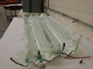
Figure 4: Vacuum wrapping of the 2nd
beam’s two halves.
Then a piece of pre-impregnated carbon fiber mating is trimmed to the approximate lengths and widths equal to the dimensions of each the tubing. Each piece is set into its respective aluminum molds and surrounded in a vacuum bag. A vacuum is drawn into the bags compressing the carbon matting to the mold. This removes air bubbles and assures a successful model.
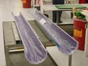
Figure 5: Two cured halves of the 2nd
beam.
The two loaded molds are then placed into an autoclave. This is a vessel used for curing fiber resin composites and is used to control the composites surroundings ensuring optimal curing conditions. Once cured the composite half tubes are trimmed to a length of 56 inches and an external radius of 3 inches. Before attaching the two halves, two gang channels and four bulkheads are installed onto one-half. The gang channels are made up of a 2-inch wide, 56-inch long flat piece of aluminum with paired fasteners running longitudinally and are used to connect the two halves. The bulkheads are hydro formed from a 6061 aluminum alloy. The dies used for the hydro forming were designed on a CATIA 3-D design package and created by stereo lithography. Three of bulkheads are installed, beginning at the leading edge, at 5 inch spacing and support the 1st beam.
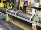
Figure 6: Intermediate joint between the 2nd and 3rd beam.
The last of the four bulkheads is installed at the trailing edge and gives support to the end of the 2nd beam.
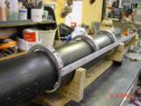
Figure 7: 3rd beam internal
bulkheads.
The gang channels and bulkheads are installed and the two halves are sandwiched together using special aviation fasteners. These fasteners resemble fine thread screws, but are mad of titanium and have a directional, offset Phillips head pattern. For the 3rd beam the same processes are used with the exception of the outer diameter and the bulkhead spacing. Instead, this 3rd beam has an outer diameter of 8 inches and a bulkhead spacing of 12 inches, while still maintaining the 56-inch length. With the three beams fabricated, they are ready for assembly. Beginning with first two beams, slide the 1st beam into the 2nd beam’s foremost bulkhead and continue until the beam passes through the second and third bulkhead. This is done until no more than 48 inches of the 1st beams length is visible from the first bulkhead of the 2nd beam. These same steps are repeated until no more than 31 inches of the 2nd beam are visible from the leading edge of the 3rd bulkhead. At this time the beam assembly is considered to be at its fully extended position and is ready to be inserted into the mounting jig. The mounting assembly was also designed using a CATIA 3-D design package.
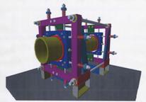
Figure 8: CATIA 3-D drawing of the mounting
jig assembly.
The intent of this mounting fixture was to eliminate movement in the longitudinal direction (z), but allow movement in the x and y directions. The mounting fixture is made up of two mirrored pieces comprised of a front and a rear. Examining the front portion of the fixture reveals three main pieces, an inner collar, an inner frame and an outer frame all sharing a consistent depth of 2 inches.
Figure 9: Closer look at the inner collar
of the mounting jig assembly.
The inner collar is made up of four curved pieces roughly a ½ inch thick with the inner diameter being adjustable from 9 inches to less than 8 inches. These four pieces, when in place, hold the beam assembly in place. The collar pieces are attached to the inner frame by four 3/8 inch threaded rods 2 ½ in length. The inner frame is a 12 by 12 inch square 2 inches thick with a centered 10-inch diameter hole cut out. Each external corner of the internal frame has been mortised to allow a ½ bolt to be pinned 2 inches from each edge of the square. These eight ½ inch threaded rods are 8 inches long and have machined flat spots on the last 2 inches of the bolt. The flat spots permit the bolts to fit into the mortised hole in the inner frame and pass through the outer frame. The outer aluminum frame is made up of an overall outer dimension of 24 by 24 inch square, 2 inches thick and an inner dimension of 20 by 20 inches. Each of the eight threaded rods extend beyond the outer frame and have spacers inserted between the outer frame and the end of the rods. Changing the type of spacer used allows for known and controlled variable end mount flexibility. This allows for reproduction of many endpoint-mounting configurations. After spacer selection a special encapsulating washer, washer and nut are used to fix the two portions of the frame together. Three different types of spacers are used a solid aluminum round spacer, a set of stiff springs and a set of weaker springs. Along with the Teflon strips attached to the outer frame, as a guide for the internal frame, additional pieces are welded to the structure to ensure even less movement in the z direction. Extra aluminum was also added to elevate the structure enough to allow access to the mounting bolts. The mounting bolts are used to attach the fixture to the shaker table. Once both front and rear portions are assembled, they are attached to each other by four threaded rods ¾ of inch in diameter and 28 inches in length with a fastener sandwiching both front and rear portions of the fixture. The beam assemble is ready to be mounted to the end fixture. Sliding the 3rd beam of the beam assembly into the front and then the rear portion of the assembly until 33 inches of the 3rd beam is extended out frontward beyond the face of the front fixture assembly. The entire system is assembled and suitable for dynamic testing.
Figure 10: Completely assembled beam
mounted to the MTS shaker table.
Test
Equipment
To determine the harmonic vibration signatures of the system dynamic testing are performed using a Material Testing System (MTS) shaker table. The shaker table introduces vibration by using a large hydraulic cylinder and pump controlled by an open loop data acquisition system. This forces the fixture vertically at specified frequencies and amplitudes. Based on user-entered parameters ranging from test time duration, displacement or acceleration and frequency, a control circuit regulates the pressure and direction of the shaker table. By continuously monitoring the table’s position and acceleration via an accelerometer mounted to the belly of the shaker table, a close relationship is maintained between the output signal to the table and the actual table response. To minimize inaccuracies occurred during short and long duration testing the MTS shaker table is mounted to an isolated slab 10 feet wide in both direction and 12 feet deep and has a liquid cooled hydraulic system.
Data
Acquisition
For data collection the acquisition
system consisted of two main groups of equipment: the accelerometers and a signal processing
system. Since this research is being
used to correlate Gulfstream’s finite element analysis data with
Before testing can begin a means to record vibration data is needed. For the purpose of this research a total of 12 PCB piezoelectric accelerometers were used. A piezoelectric accelerometer is a device that uses crystals to measure the acceleration.

Figure 12- PCB 353B03 accelerometer.
This works by sandwiching a crystal between the accelerometer housing and an internal mass, once a change in velocity takes place the crystal is deflected or distorted. By knowing much force is required to deflect a crystal a given distance and the amount of internal mass, the force can be related to acceleration as a voltage [17]. The 12 Piezotronics, Inc accelerometers used in this research were made up of a mixture of eight Integrated Circuit Piezoelectric (ICP) single axis accelerometers (PCB model number 353B03) and 4 tri-axial (ICP) accelerometers (PCB model number 356A02). PCB Internal Circuitry Piezoelectric accelerometers have the following general characteristics: fixed voltage sensitivity, low-impedance output signal, two-wire operation, low-noise, voltage-output signal and an intrinsic self-test feature [14]. The accelerometers were attached to the test specimen through mounting pads. The mounting pads are made of ¾ inch round stock and cut to 3/8 inch thick. They are tapped to accept accelerometers and one of the flat surfaces is machined to match the beams curvature enabling a tight mount. After attaching the accelerometers to the beams a cable individually transmits each of the accelerometers vibration information to a system designed to process the accelerometers’ signals.
The accelerometers by themselves are
incapable of supplying understandable frequency results if capable of supplying
anything at all. In order to render
these devices useful, the raw information read from the accelerometers must be
fed, read, processed and stored before receiving satisfactory frequency results. For the purpose of this research these
processes were performed using technology from National Instruments™. Their data acquisition system consisted of a
SCXI-1001 chassis, three SCXI-1531 analog input modules, a PCI-MIO-16E-1 DAQ
and LabVIEW™ for Windows. These devices
worked simultaneously in unison to processes the various signals.
Independently, the accelerometers do
not send out any information, because they require a power supply. Their power is supplied through three
SCXI-1531 analog input modules which are mounted to and supplied power from the
SCXI-1001 chassis. Once everything is in
place and power is supplied the accelerometers are capable of sending
information in the form of voltage. At
this time the voltage signals need to be converted in a way that is
understandable by the computer and able to be converted to acceleration. In order to successfully achieve this, SCXI-1531,
PCI-MIO-16E-1 DAQ and LabVIEW™ must work together in harmony. The SCXI-1531 modules take and condition the
signals arriving from the accelerometer.
Each module is capable of handling eight accelerometers. The first slot was set up to handle a single
axis accelerometer (PCB model number 353B03), while the following two slots
were set up for four tri-axial accelerometers (PCB model number 356A02). Each of these modules was proficient enough
and programmable to control current, gain, and filter settings on each
channel. These modules also feature
simultaneous sample-and-hold circuitry (SSH) [15].
The next step is for the PCI-MIO-16E-1
DAQ to read, convert, process and send information based on the instructions
given by LabVIEW™. It achieves this by
multiplexing the numerous voltage signals entering from the three SCXI-1531
analog input modules. While entering the
PCI-MIO-16E-1 DAQ the signal is filtered and converted to binary code where it
waits shipment to the computer. Table 1 lists
the hardware components of the data acquisition system [14,15]:
Table 1: Data Acquisition
System configuration
|
Item |
Qty. |
Mfg. |
Part Number |
Description |
|
01 |
1 |
National Instruments™ |
776571-01 |
SCXI-1001,
12 Slot |
|
02 |
3 |
National Instruments™ |
777966-31 |
SCXI-1531 8-Channel ICP Accelerometer Module, BNC Connectivity |
|
03 |
1 |
National Instruments™ |
777305-01 |
NI PCI-6070E (PCI-MIO-16E-1) DAQ Device |
|
04 |
1 |
National Instruments™ |
776574-492 |
SCXI-1349 Shielded Cable, 2m |
|
05 |
8 |
PCB Piezoelectric, Inc. |
353B03 |
ICP Single Axis Accelerometer |
|
06 |
8 |
PCB Piezoelectric, Inc. |
356A02 |
ICP Tri-Axial Accelerometer |
|
07 |
4 |
PCB Piezoelectric, Inc. |
002C10 |
Coaxial Cable 10-32 Plug/BNC Plug |
|
08 |
4 |
PCB Piezoelectric, Inc. |
010G10 |
Cable Assembly (4-Pin to 3 BNC Connectors) |
Manipulation
The information collected by the accelerometers and processed by the data acquisition systems exits in an unrefined form and is saved as an American Standard Code for Information Interchange (ASCII) file. For each of the 12 accelerometers there exists a large file of frequency versus time data. At this point each of the file’s information is confusing, because there are shifts in the phasing between accelerometer information due to their locations. In order to make sense of the information the data is reorganized by Diadem 8.1. This is a tool for graphing and manipulating large files. The next step is to take the ASCII file and import it into Diadem 8.1. Once imported into diadem the information is more meticulously filtered and a Fast Fourier Transform (FFT) is performed resulting in a graph of amplitude versus frequency. From the frequency spectrum graph resonant frequencies are evident by their large relative amplitudes and appear as spikes on the graph.
Testing
Testing consisted of three separate sets of tests. The first test set is used to establish the affects the main fixture’s flexibility as an end mount has on 1st and 2nd modes of resonant frequency. The second set of tests explores the changes to the 1st and 2nd resonant frequencies due to intermediate joint flexibility between the 1st and 2nd beam by varying the bulkhead arrangement. Separately the second test group explores the relationship between the 2nd and 3rd beams joint stiffness on the 1st and 2nd natural frequency. The final set of tests looks at the relationships between the retraction/extension lengths of each of the beams segments and their respective 1st and 2nd modes of resonant frequency. For each of these last tests three separate methods of retraction/extension are considered.
Main
Fixture
Testing begins by attaching the mounting jig to the shaker table. This fixture consists of four main parts a front and rear section with both internal (main fixture) and external portion (8-inch collar supporting fixture). For each of the front and rear sections eight spacers attach the internal and external portions to each other. These spacers are selected based on test requirements. For the first test solid round aluminum spacers (SRAS) are used to attach the internal and external portions together yielding a spring constant k = 1.733 x 10⁶ lbs/inch for each bulkhead section. This is used to represent a rigid connection within the jig bulkhead. These front and rear internal portions of the fixture attach to the largest of the three-cantilevered beams in two places. The spacing between these two points can be arranged from 24 inches to 12 inches in 6-inch increments. For the first test the fixture is attached to the table with 24-inch spacing. The largest beam is the beam with 8-inch diameter; it is attached with the leading edge of the beam extending 27 inches out of the fixture. From this leading edge the second largest beam, the beam with the 6-inch diameter, is extended 31 inches outward. Then from the second leading edge the smallest 2-inch diameter beam is extended outward 48 inches. With the beam mounted securely to the fixture with each of beam lengths fixed the accelerometer mounting pads are installed. For simplicity the x-axis is positive upwards in the vertical and the z-axis runs positive out towards the leading edge. There are five mounting pads attached to beam 1. The first mounting pad is attached to the trailing edge of beam 1, perpendicular to the top edge of the beam in the XY plane, and the remaining four are evenly spaced on the upper side of the cantilevered section in the XZ plane. Once these pads are attached to the beam using Loc-Tite the accelerometers are threaded into the mounting pads. Considering the leading edge of the front jig mount to be the zero point the mounting pads and accelerometers are arranged as follows:
|
Mounting pads &
Accelerometers |
Location |
Distance |
Type |
|
1st |
Trailing edge |
-27 inches |
Tri-axial |
|
2nd |
Top |
0 inches |
Tri-axial |
|
3rd |
Top |
9 inches |
Uni-axial |
|
4th |
Top |
18 inches |
Uni-axial |
|
5th |
Top |
27 inches |
Tri-axial |
Table 2: Beam 1 mounting pad and
accelerometer location.
For beam 2 the mounting pads and accelerometers are attached as follows:
|
Mounting pads & Accelerometers |
Location |
Distance |
Type |
|
6th |
Top |
28 inches |
Uni-axial |
|
7th |
Top |
37 1/3 inches |
Uni-axial |
|
8th |
Top |
47 2/3 inches |
Uni-axial |
|
9th |
Top |
58 inches |
Tri-axial |
Table 3: Beam 2 mounting pad and
accelerometer location.
For beam 3 the mounting pads and accelerometers are attached as follows:
|
Mounting Pads & Accelerometers |
Location |
Distance |
Type |
|
10th |
Top |
59 inches |
Uni-axial |
|
11th |
Top |
82 inches |
Uni-axial |
|
12th |
Top |
106 inches |
Uni-axial |
Table 4: Beam 3 mounting pad and
accelerometer location.
After
attaching the mounting pads and accelerometers, wires are run from the ADC to
the accelerometers. Beginning with 12th
accelerometer and ending with the 1st fill the first slot (0-7) of
the ADC with the eight uni-axial accelerometers and then fill the 2nd (8-15) and half of the last slot
(16-19) with the tri-axial accelerometers.
After securing beam to the jig assembly, fixing each of beam lengths,
attaching the accelerometer mount pads and accelerometers set the MTS shaker
table, for group 1 testing, to scan from 10-70 hertz at .5 g’s. The intensions of these tests are not to
destroy the test specimen, but to simply single out frequencies of
excitation. The MTS shaker table is
setup to introduce vibrations in the X direction.
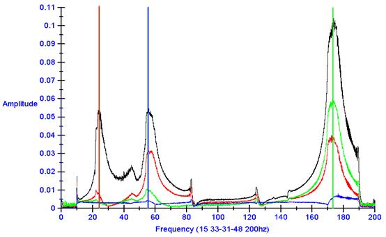
Figure 14: Resonant frequency scan at fully
extended.
After the test is run and the data is collected from the accelerometers the information is exported into Diadem and converted from “displacement vs. time” information to “amplitude vs. frequency” by performing a Fast Fourier Transform (FFT). The first and second natural resonant frequencies appear as spikes and are located where the derivatives are zero or at the point of inflection. This is considered Test 1A. In Figure 14 the 1st resonant mode is represented with a vertical red line, the 2nd a blue line and the 3rd. The vertical lines were roughly set into position by location the center of the highest point.
HSS/Spacing
With everything remaining in the same position, replace the round aluminum spacers (SRAS) in the mounting fixture with the Heavyweight Spring Spacers (HSS). The HSS are used to represent a semi-flexible jig bulkhead with a spring constant k = lbs/inch per bulkhead section. The SRAS are removed by placing two 2-inch spacing blocks in the front bulkhead jig between the lower internal and external fixtures and two 2-inch cube spacing blocks in the front bulkhead jig between the upper internal and external fixtures. Then the retaining nuts are removed along with the solid spacer washers and solid spacers. The internal portion of the fixture is freed from the external portion of the fixture and completely rests on four 2-inch spacing blocks. Begin with the upper front pair of spacer mounts and the rear lower pair of spacer mounts and replace the SRAS with the HSS. Then tighten the fasteners in pairs until the internal fixtures release its respective pair of 2-inch cube spacing blocks enough to permit effortless movement. Once the blocks are freed, begin installing the springs on the opposite side of the same bulkhead jig. Again in pairs tighten the fasteners until the internal and external fixtures slightly pinch the blocks prohibiting movement then back off the fasteners just enough to release the blocks. Repeat these steps for the side spacers working in opposites from front to back until all of the HSS are installed. Finally, preload the springs by tightening each of the fasteners an extra 1 ½ turn. This is considered Test 1B.
LSS/Spacing
The third test involves replacing the eight front HSS and eight rear HSS with the 1.5-inch diameter light spring spacers (LSS). The installation method for these will use the same steps as mentioned for the HSS. Once installed the spring constant for each of the bulkhead fixtures is 5120 lbs/inch. This is considered to be Test 1C and will conclude the variable end stiffness testing for a 24 inch main fixture spacing.
|
Test name (@ 24-inch MFS) |
Spacer Type |
|
Test 1A |
Solid (SRAS) |
|
Test 1B |
Heavyweight Springs (HSS) |
|
Test 1C |
Lightweight Springs (LSS) |
Table 5: Test name of fixture spacer
selection at 24 inch Main fixture spacing.
The next group of tests, within set one, involves moving the front jig-mount fixture back from 24 inch spacing to 18 inch spacing. Without relocating the mounting pads and accelerometers, loosen the four locking nuts surrounding the front 8-inch diameter collar located in the internal portion of the front fixture. Then back out the four, collar adjustment studs that attach collar to the 1st beam. This is done to allow movement of the front jig mount. With the front collar loosely surrounding the 1st beam completely remove the bolts that mount the front external fixture to the table and loosen the rear external fixture bolts ½ of an inch. With everything loose, begin to retract the front jig mount by turning the fasteners located in each corner of the front jig mount. This is done until the front jig mount holes align with the holes in the shaker table. The holes in the shaker table are located every 6 inches. Having aligned the front fixtures holes with the next set holes in the table, the total fixture spacing is moved from 24 inches to 18 inches. With the bulkhead spacing moved from 24 inches to 18 inches, replace the fixture to table bolts and tighten. At this point all of the procedures for replacing the SRAS, HSS and LSS performed for Tests 1A, 1B and 1C at 24-inch main fixture spacing are repeated for the 18-inch spacing. This is considered to be Tests 1D, 1Ea and 1Eb and will conclude the variable end stiffness testing for an 18-inch main fixture spacing.
|
Test name (@18-inch MFS) |
Spacer Type |
|
Test 1D |
Solid (SRAS) |
|
Test 1Ea |
Heavyweight Springs (HSS) |
|
Test 1Eb |
Lightweight Springs (LSS) |
Table 6: Test name of fixture spacer
selection at 18 inch Main fixture spacing.
The last of three of the nine
variable end stiffness tests is conducted at a main fixture spacing (MFS) of 12
inches. At this spacing each of the
three different spacers are replaced, tested and named as follows:
|
Test name (@12-inch MFS) |
Spacer Type |
|
Test 1F |
Solid (SRAS) |
|
Test 1G |
Heavyweight Springs (HSS) |
|
Test 1H |
Lightweight Springs (LSS) |
Table 7: Test name of fixture spacer
selection at 12 inch Main fixture spacing.
From all of these nine tests a 3 x 3 matrix of variable endpoint stiffness is constructed based on FFT 1st and 2nd mode natural resonant frequencies. These are used and compared to the model being constructed for validity.
Intermediate
Joint Arrangements
Joint
1-2
The second batch of tests analyzes the relationship between resonant frequencies and joint stiffness between the beams. For these tests, the main fixture’s spacing is returned to 18 inches and the SRAS are used instead of the springs. The 18-inch spacing is used since it is the end fixture’s mid setting for collar spacing and the springs are not used to eliminate the potential of changing data due to relaxing springs. The first joint is considered the area at which the 1st and 2nd beams attach to each other. In the interior of this first joint exists a series of bulkheads, originally setup as a default setting of 3 bulkheads D, E and F with a spacing of 12 inches between the bulkheads. They are arranged according to the following test requirements:
|
Test name (@18 inch MFS) |
Bulkhead location |
|
Test 2A |
Baseline Configuration |
|
Test 2B |
Remove Bulkhead e, keep f |
|
Test 2C |
Move Bulkhead f to second
position |
|
Test 2D |
Remove bulkhead f, keep e |
Table 8: Test name and bulkhead location.
Joint
2-3
The second test performed within group 2 testing is the examination of the joint stiffness between the 2nd and 3rd beams known as the second joint. These tests are performed with joint 1 returned to its default configuration. As a default the second joint consists originally of three bulkheads A, B and C. They are arranged as follows:
|
Test name (@18 inch MFS) |
|
|
Test 3A |
Baseline Configuration |
|
Test 3B |
Remove Bulkhead b, keep c |
|
Test 3C |
Remove Bulkhead c, keep b |
Table 9: Test name and bulkhead location.
Extension/Retraction
Extending Beam Three 1st
Test group 2 explores the contributing affects that retraction and extension have on the systems natural frequencies. It is also a tool for comparing the different possibilities of retraction and extension. The first test of this kind examines the changes in natural frequencies based on the smallest (3rd) beam extending first, the medium (2nd) beam and then the largest (1st) beam. This is the same as retracting the 1st beam first, 2nd beam next and the 3rd beam last. In order to minimize the number of tests, each beam is retracted or extended in 4-inch segments unless more information is needed in an area. First, all of the beams are extended to what is considered fully retracted. For this system, the 1st beam is extended until its tip is 33 inches from the face of its respective supporting end bulkhead, the 2nd beam at 31 inches and the 3rd beam at 48 inches. Then with the 4 sensors in place, a test will be run, scanning from 10 Hz to 70 Hz. For these tests, a single sensor is mounted on the top portion of each beam near the leading edge and the fourth sensor is mounted on the top portion of the trailing edge of the 1st beam. This is found on the rear side of the main mounting fixture. After this test is run and recorded, the 1st beam is retracted 4 inches, run and recorded. It is the testing operator’s responsibility to frequently monitor the scan range, because as the beam retracts it is possible to chase the resonant frequency out of the scanning range. It is left to the operator to select the correct scan range based on observations. This procedure is sustained until the 1st beam is considered fully retracted. For this system, each beam is retracted no more than 1-inch from the face of its respective supporting end bulkhead. More clearly, this states that for any of the 1st, 2nd and 3rd beam to be considered fully retracted they must have only 1-inch extending out of its respective visible support. After running and recording the 1st beam at 1 inch and the other two beams fully extended, repeat the retracting procedure for the 2nd beam. As for the 1st beam, the 2nd beam is only retracted until 1 inch of the 2nd beam remains extended beyond its visible support. After this is tested and recorded the same procedure is repeated for the 3rd beam. This concludes the frequency testing of the outer, center to inner (OCI) retraction method.
Equally
Extending Beams
While leaving the sensors in the same location the beams are fully extended, a different method of extension and retraction is tested. The next test of group 3 testing considers a concentric method of retraction and extension. Test 3 explores the resonant frequency possibilities experienced while extending or retraction the three beams equally. Begin by dividing each beam into segments. The number of segments for each beam does not matter, but must be the same for all three beams. Increasing the number creates more tests, but gives more clear results. While the beam is fully extended, another test is run and recorded. The earlier test for fully extended could have been used, but by retesting the same point repeatability can be shown. Next, each beam is retracted to its first mark. None of the beams retraction lengths are the same, but the ratios of retractions are meaning that when the beam does reach full retraction all three beams will be retracted. For each retraction a test is run and recorded, this is repeated until the beam is fully retracted.
Extending
Beam One 1st
The last test considers the final possibility of retraction where the beam could be retracted from inner, center to outer (ICO). The procedure for retracting (ICO) is the same as (OCI) except the order of beam retraction is reversed. For this test, the first beam retracted is the inner beam, then the mid beam and finally the outer most beam. In between each retraction, a test is run and recorded. This concludes the testing for group three.

Figure 15: Fully extended beam mounted to
the MTS shaker table.
Results and Discussion
![]() Equation
9
Equation
9
![]() Equation
10
Equation
10
![]() Equation
11
Equation
11
 Equation
12
Equation
12
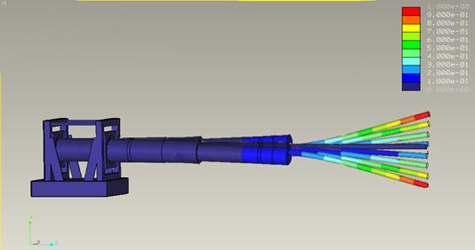
Figure 16: 1st resonant mode FEA
model.
The legend in the upper right hand corner represents the amount of deflection based on colors. The bluish colors represent the least amount of deflections while the reddish colors represent the most deflection. Although the 1st mode displacement is clearly visible during testing, for the purposes of display the deflections have been scaled for exaggeration. For the 1st mode of frequency there is not any point of inflection and the beam continually deflects more towards the free end of the beam.
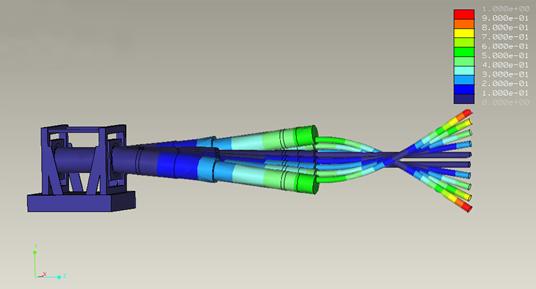
Figure 17: 2nd resonant mode FEA
model.
Figure 17 is Pro-Mechanica’s representation of the 2nd resonant mode. By taking a closer look at the model’s 2-3 joint a single point of inflection is evident. Although simply having a single point of inflection does not specify that this is the 2nd resonant frequency it only states that it is not the 1st or 3rd. By looking at the shape of the beams a near ¾ sin wave can be seen and now has two large areas of displacement as opposed to the 1st resonant frequency’s one. While running through these frequencies on the test, these frequencies were not as visible as the 2nd mode frequencies.
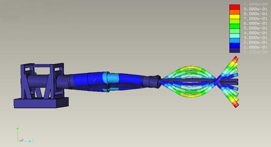
Figure 18: 3rd resonant mode FEA model.
For all tests, the same USC-FEA model is used as a comparison of measured test results. Using the FEA branch of ProE known as Pro-Mechanica a duplicate model is created. Each beam is created using similar dimensions of lengths, diameters, bulkhead locations, materials, densities, and stiffness. In addition, the model incorporates an end main fixture with all of its dimensions and properties. Young’s modulus is found by using experimental deflection data with their respective applied forces. Clamping the smallest beam (beam 3) to a table so that 29.5625 inches cantilevers out past the end of a table, the following loads are applied to the end and the deflections for each of the loads are measured at the end.
|
Mass (grams) |
Deflection (inches) |
|
2455.7 |
0.0388 |
|
2908.6 |
0.0450 |
|
3361.6 |
0.0530 |
|
3814.7 |
0.0620 |
|
6079.4 |
0.0995 |
Table 10: Mass applied and respective
deflection.
Converting the units and using the equation of bending for a cantilevered beam with a concentrated point mass:
![]() Equation
13
Equation
13
Where:
![]() Equation
14
Equation
14
Plugging equation 14 into equation 13 with all known constants and evaluating the deflection at the end yields a Young’s modulus of 38.63 gigaPascals (GPa). Finding the mass of the same beam and dividing by the volume gives the density of the material to be 1319.247235 g. This same model is run through all of the tests that the actual quarter scale model is run and compared with the exception of those tests requiring stiff and light springs. The model is not perfect and FEA testing with springs in place of SRAS crashes. A possibility for future research should include an improved model with the ability to incorporate the use of springs as spacers.
Main
Fixture Spacing
The first sets of tests are constructed of main fixture spacing and spacer type. For these tests, the beams are each fully extended giving an overall length of 112 inches.
Figure 19: 1st Resonant Frequency
vs. Main Fixture Spacing
Figure 15 examines the 1st resonant frequency response changes in equidistant bulkhead spacing and spacer selection yield nearly linear results within each spacer type selected. As expected with an increase in the main fixture’s rigidity the 1st resonant frequency also increases as seen in the graph. Representing the lowest tested main fixture rigidity is the red line, the central the blue line and the highest possible main fixture rigidity is the green line. Within each of these lines are three points, which represent the main fixture spacing. These points represent, from left to right, an increase in end mount rigidity associated with a larger main fixture bulkhead spacing. This creates a larger footprint to counter forces presented by beam during excitation forces. In addition, the USC-FEA model produced similar results for SRAS at all three main fixture spacing.
Figure 20: 2nd Resonant Frequency
vs. Main Fixture Spacing
Results found for the 2nd resonant frequency in Figure 16 are similar to the trends found in 1st resonant frequency. As expected with an increase in the main fixture’s rigidity the 2nd resonant frequency also increases as seen in the graph. From lowest 2nd mode of resonant frequency to greatest is the red line, the central the blue line and the highest possible main fixture rigidity is the green line. As stated earlier, the red line represents the springs with the smallest K, blue represents the stiffer springs, and the green line represents fixture with the SRAS. The black line represents the USC-FEA model, with SRAS, and reproduces frequency increases and changes in slope comparable to actual quarter scale test results.
Figure 21: FEA and Model Comparison
Intermediate
Joint Arrangements
Joint 1-2
Figure 22: 1st Resonant
Frequency vs. Bulkhead Position
By comparison, the graph’s nonlinear decreasing slope is visible in the green line. This represents a decrease in 1st mode resonant frequency and matches the effects of the decreasing stiffness on a beams resonant frequency. Although examination of the 1st mode frequency response predicted by the FEA model, represented by a red and blue line, illustrates a decreasing slope with lower values it appears to be somewhat linear. If this were just a matter of slightly lower FEA results the problem could be fixed by modifying bulkhead material properties, but the fact that there exists unrelated slopes this represents a probable flaw in the FEA model’s ability to accurately recreate the quarter scale model’s intermediate joint stiffness and may be the cause for dissimilar results in future tests. The next graph presents the results for 2nd resonant mode responses. These tests results follow the same trends as shown earlier in the 1st mode graph with the exception of test 2C of the recorded second mode information represented by the green line. For the 2nd mode of test 2C the test results match closer to the FEA model’s results for 2C these are represented by the red and blue lines. After test 2C the FEA model remains on a linear path while the tested quarter scale model slope decreases to the point where it actually crosses the FEA results.
Figure 23: 2nd Resonant
Frequency vs. Bulkhead Position

Figure 24: Bulkhead position model
comparison
Joint 2-3
The next subset test set 2 examines the joint between beam 2 and beam 3. While examining this subset of tests, the joint between the 1st beam and the 2nd will be left in original Stock orientation.
Figure 25: 1st resonant
frequency of 2nd beam bulkhead position
Figure 26 was arranged in way such that the strength of the 2-3
joint was decreased. This is evident by
the decreasing value of the 1st resonant frequency from left to
right. It is clear to see by this same
figure that the joint internal structure is not understood by the USC-FEA
model. Out of three internal bulkheads
two of them were moved around giving the three different arrangements 3A, 3B
and 3C. Although the changes were
substantial when viewed by the quarter scale model, the USC-FEA model remained
relatively unchanged. If a line were fit
through the models data it would almost be parallel, whereas for the quarter
scale model there would be considerable slope.
This is the second test that showed undesirable results when comparing
to the USC-FEA model.
Figure 26: 2nd resonant frequency
of 2nd beam bulkhead position
The second resonant frequency results for 2-3 joint testing shows to be more promising. As seen in Figure 27 the trends are more similar than they were in Figure 26. If for this graph a line were fit through all three data sets they would be more parallel than before. Although the frequency values are not the same the trends are, and again as seen in Figure 28 the 2nd resonant frequencies are closer to the quarter scale model than the 1st resonant frequencies.
Figure 27: 2nd beam model
comparison of bulkhead position
For Figure 28 the 2nd mode never gets further than 4.34%
away from the quarter scale model’s results while for the same bulkhead
position the 1st frequency reaches 15.57%. These results are similar to those found
within 1-2 joint testing, where there too the 2nd mode was more
correct than the 1st mode. As
the beam’s joints were made less stiff they comparisons between the two models
worsened beginning from the 1st test 3A the difference between the 1st
and 2nd mode are 1.14% while the 2nd is 3.19% and then
the last test gives the worst results of 11.23%.
Original Retraction/Extension
Tests
Extending Beam 3 First
Figure 28: Resonant frequency vs. Extension
from beam 3-1
As a function of length, the solid red line represents the 1st resonant modes of the USC-FEA model and the red crosses represent the quarter scales 1st resonant modes. The 2nd modes are represented as the same for the blue line and crosses and the green line and crosses represent the 3rd modes for USC-FEA and quarter scale model respectively. Reiterating the earlier statement where the most important modes examined are the 1st and the 2nd modes any other modes captured were not intended, but still remain helpful in model validation. Of the two intended modes, the 1st natural resonant frequency is the most important since the object is to obtain the lowest mode possible and force that mode out of the planes range which is low on the scale. By looking at Figure 24 the most blatantly obvious information retrieved from the graph is the affect the smallest beam has on the 1st mode. As the beam extends the resonant frequency increases until it reaches its max of 105 Hz at 26 inches of length then the resonant frequency begins to fall. Knowing that neither the 1st nor the 2nd beams are ever retracted to more than 1 inch it is understandable that this maximum 1st mode resonant frequency is located at the midpoint of the third beams extension. Looking from 2 inches to 50 inches of extension it is also discovered that this is same point at which the 1st mode resonant frequency appears to symmetrical. Therefore, for this method it appears that the greatest affect on the 1st mode resonant frequency is the movement of the smallest beam.
As stated earlier this is the last of the tests performed; this is mostly visible near the fully retracted region. Early tests recorded near the fully retracted area of the graph are noisy and some of the frequencies are indistinguishable, but as testing practices improved so did the ability to read small extension frequencies even though they may display large discrepancies between the models.
Figure 29: FEA and model comparison vs.
length
Visible in the Figure 25 is the close similarity between all 1st modes of the USC-FEA model and the quarter scale model. Figure 25 represents the absolute value of the percent difference between the actual quarter scale model testing and USC-FEA as a function of overall length. The next important resonant frequency is also the next closest in comparison as far as trends go. Acknowledging that the 2nd is not perfect throughout the range of the extension lengths, it is an excellent indicator of the 2nd mode trends exhibited by the quarter scale model. This was and still is the original intent of the USC USC-FEA model without which would have resulted in an inaccurate selection between 1st and 2nd resonant modes. A comparison of 3rd resonant modes reveals similar trends between both of the models. One thing quickly observed from Figure 25 is that for most of the graph two resonant frequencies trends tend to act accurately or inaccurately together. It is possible that a joint is not represented accurately by the model and is something that would need to be addressed for future research. Even with most of the error being less than 12% for the 1st mode, there is need for improvement within the model.
Equally Extending
Figure 26 represents the resonant frequency versus the total length of the three beams, as the three beams extend and retract equally. It is clear to see some symmetry in the graph about the 56-inch mark for the 1st mode of resonant frequency. This is points represents ½ of full extension or retraction length. The beginning and ending frequencies are 28.89 Hz and 30.65 Hz respectively and are different by less than 2 Hz.
Figure 30: Resonant frequency vs. Equal Extension
of Beams
By looking at the information in the graph, it can be justified that for this system the mass and stiffness properties behave symmetrically, about the 56-inch mark, during an equal extension or retraction rate, but if this is the exact case why would the 2nd and 3rd only show a similar trends without similar frequencies. Although this topic is not studied within this research, it presents an interesting question pertaining to the differences between 1st, 2nd and 3rd mode resonant frequencies. 1st resonant modes for cantilevered beams are represented, pictorially, by a single node located at the fixed point and an anti-node located near the free end of the beam. It is possible for many dissimilar mass and stiffness systems to give similar 1st mode resonant frequencies such as the three beam system when it is fully extended and fully retracted. The 2nd resonant mode is represented, pictorially, by 2 nodes and 2 anti-nodes. The 1st node and the last an anti-node are respectively located at the fixed end and the free end, as stated earlier, but the inner node and anti-node are able to move back and fourth relative to mass and stiffness relationships. It would seem more commonplace for a node and anti-node to be located nearer to these intermediate joints since these represent some point of inflection along the beams. Since this is not an isotropic or homogeneous beam and the joints are located very differently between fully extended and retracted, it appears to be less probable for the 2nd modes to be symmetrical with respect to both trends and Hz. It appears, that with an additional node and anti-node for the 3rd resonant frequency, that the 3rd mode is more symmetrical than the 2nd mode relative to Hz, but has shifted its axis of symmetry about the 63-inch mark. This is complicated information that needs to broken off into a separate research topic of its own.
Extending Beam 1 First
This section covers the extension method by which the largest beam extends first and concludes the study on the different methods of retraction. Although this is the last of the methods explained, it was actually the first tested and evident by the lack of data points recovered within the early testing stages of extension of Figure 27. For this early set of tests both the tested quarter scale model and the USC-FEA model are missing points. No modifications were done to the model to improve results, just the method of compressing the information retrieved. Illustrated in Figure 27 is a large gap in points for the 1st mode of resonant frequency running from 0 to 32 inches. Within this area the resonant frequency was so low that it blended into the lowest tested frequency tested. Earlier there was mention of the shaker table’s inability to test low frequencies below 10 Hz. During extension of the quarter scale model within the 0 - 40 inch extension region the 1st resonant frequency disappeared into the no-test zone, was indistinguishable from noise and was left blank. Oddly enough, the USC-FEA model’s 1st mode resonant frequency flattened out, but where exactly was not determined from the results. Having proved the USC-FEA model’s ability to reproduce the quarter scale model results accurately leads to speculate that it is very likely that the 1st mode of the quarter scale model plateaus from 0 - 40 inches below 28 Hz.
Figure 31: Resonant Frequency vs. Beam
Extension 1-3
For 1st resonant modes less than 40 inches Figure 27 can only serve as an upper bound for the lowest resonant frequencies. We have to assume the worst since the largest concentration of this work is focused on the lowest resonant frequencies and the frequencies are lost into the lowest frequencies for this set of tests. Although not as important, the trends for the 2nd and 3rd resonant frequencies were just as accurately represented by the USC-FEA model.
Beyond 40 inches of extension and closer to the 62 inch mark begins the end of the flat 1st resonant frequency trend. This begins the extension of the smallest of the three beams which is beam three. By examining the 2nd and 3rd modes the point of inflection lies at the midpoint of the smallest beam. This was the same trend produced when the 3rd beam was extended first. By association these two tests insinuate that the smallest beam, beam three, is the largest contributing factor to resonant frequency changes to the 1st resonant mode within this particular system.
Figure 32: FEA and Model Comparison vs.
Length
Although the similarities between both the USC-FEA and quarter scale models are uncanny there is a lack of increase in resonant frequency associated with retraction of typical cantilevered beams. Of coarse any variation in the retraction or extension order would not change the endpoint resonant frequencies, but it was not obvious that the beginning and ending lowest resonant frequency would be within 2 Hz of each other. This is caused by the lack of support within the beams for the unexposed portions of the beams. When going from fully retracted to full extension the beams only swap which of the ends are cantilevered and is evident by the symmetry of resonant frequencies within Figure 24, Figure 26 and Figure 27. Stopping research at this point suggests there is no best method of retraction/extension to avoid low resonant frequency areas, because they all begin and end at the same location. Although obvious to begin with, tests were expected to suggest which method crossed through dangerous resonant frequencies the quickest, but instead only illustrated that all methods cross through potentially dangerous frequency ranges twice as much as originally expected.
Beam Adaptation
Unwilling to throw in the towel another approach was added to this research. Since the system is not behaving as expected the system needs to be changed. Although dampening could be used, this is the best way to avoid catastrophic failure due to vibration since dampening does not change the frequency at which a system resonates. This opened the door for the possibility of adapting the beam in order force the beam out of the low frequency ranges.
Reentering the internal structure of each of the two largest beams there are three bulkheads per beam. These three bulkheads support the adjacent smaller beam. The smallest beam three is supported by three bulkheads within the middle sized beam two. The second beam is supported by the three bulkheads within the end of the largest beam three. By attaching an extra bulkhead to the end of beam three and beam two an increase in resonant frequency can be expected due to the increased stiffness of each of the free ends. One of the bulkheads are attached at the end of the encapsulated small beam, while the other bulkhead is attached to the encapsulated end of the middle sized beam. Each bulkhead is capable of moving with each beam. Adapting the beam changes in this manner breaks up the symmetry of the mass/stiffness system throughout extension/retraction therefore changing the results of the resonant frequency for the best.
Adapted Retraction/Extension Tests
Extending Beam 3 First
Extending the smallest beam, beam three, first gave results expected when increasing the stiffness of a system without changing the mass just not in the manner expected. Since USC-FEA modeling ran quicker running from fully extending to fully retracted, it was initially thought that the USC-FEA model was not acknowledging the adaptation. It is speculation that the USC-FEA model ran faster while retracting due to the selection of the AutoGEM settings. It is a possibility that the model adapts the sections of FEA nodes as the model changes. Since at fully extended the beam’s sections internal structures are clearer for interpretation the initial AutoGEM is more accurate. It is not 100% clear and is not relevant for this research, but does explain the initial lack of confidence in early test results of the adapted beams. It was not until the beam was retracted to 83 inches that any significant changes occurred and that took place in the third mode.
Figure 33: Adapted beam resonant frequency
vs. length (extending 3-1)
Examining Figure 29 from 112 to 28 inches of retraction the first mode remained constant. Following the solid red line the changes began to transpire at the 28 inch mark. This is the point at which the solid red line leaves the dotted red line which represented the original non-adapted beam’s 1st mode of resonant frequency. The trend here was not expected as the 1st resonant mode jumped from the original 1st mode to the original non-adapted beam’s 2nd mode resonant mode. The second mode, represented in the graph by the solid blue line, momentarily left its original 1st mode while in the 73 to 50 inch extension/retraction range to mimic the original beam’s 3rd resonant mode which is represented by the dotted blue line. The 3rd resonant modes remained similar until the 83 inch mark where the trends were the same, but the values were different. They rejoined each other momentarily at the 50 and 6 inch mark.
Equally Extending
The second method of adapted beam retraction/extension is the most interesting of the three simulations run. The same mimic able trends are seen between adapted and non-adapted modes. Depending on which side of Figure 30 is looked the modes and similarities decrease or increase chronologically as the mode number increase.
Figure 34: Adapted beam resonant frequency
vs. length (extending equally)
The 1st adapted mode, represented by the solid red line, is the most similar to its previous non-adapted counterpart which is represented by the dashed red line. The adapted beams 1st mode is nearly identical to the 1st mode of the non-adapted beam from 112 to 56 inches of retraction/extension. After the adaptation of the beams, the trend is asymmetrical about the half way mark for retraction/extension, because adaptation of the beam increased the low resonant frequencies from 56 to 0 inches of retraction/extension. The 2nd adapted mode is represented by the solid green line and ranks 2nd as the most similar of the trends. This line remains over the original 2nd mode, represented by the dashed green line, from 112 to 70 inches of retraction/extension, at which this mode crosses over to the original 3rd resonant mode represented by the dashed blue line. The 3rd mode of the adapted beam matches the original beam until 86 inches. This is the point at which the 3rd beam has reached full retraction. The adapted beam’s 3rd mode trend does not return until the 1st beam begins its extension/retraction at 31 inches.
Extending Beam 1 First
This third test concludes the USC-FEA testing of the adapted beams frequency response throughout extension/retraction. After running all previous tests, it is not surprising that there are similarities between the resonant frequencies of the adapted and the original beam for this method of extension/retraction.
Figure 35: Adapted beam resonant frequency
vs. length (extending 1-3)
The 1st adapted resonant mode is represented again by the solid red line and lies directly over the original 1st mode from 112 to 72 inches of extension/retraction. At this point it crosses over and follows the path of the original beam’s 2nd mode. This is the 3rd case in which this has happened. The 2nd mode, represented by the solid green line, follows directly over the original 2nd mode from 112 to 92 inches and is represented by the green dashed line. This is again evident within the 3rd mode from 112 to 100 inches. This is the third of this type of USC-FEA testing and for all of the cases the resonant frequencies have matched for shorter lengths of retraction based on the chronological order of its frequency. The adapted beam’s 4th resonant frequency is represented by the solid orange line and only matched the original 4th mode from 112 to 104 inches which was represented by the dashed orange line.
Summary of Results
For the purposes of this research the results were satisfactory. It is clear after some two hundred different tests performed between the two models, that the results produced are valid and repeatable. For three different methods of retraction/extension and the nine various endpoint fixity conditions, the tests exposed what was not originally understood about the beams resonant frequencies. Because of this research it is known that without any adaptation of these beams they will pass through approximately the same frequencies twice for the lower more detrimental resonant frequencies. Another conclusion that can be made from this research is that the largest contributions made to the resonant frequencies result from the smallest beam, beam three. Whether seen through the USC-FEA model or the quarter scale tests, it is clear that the 3rd beam has the largest affects on setting the lowest resonant frequencies. With some adaptation of the 3rd beam resulting in a stiffer beam, the resonant frequencies could be forced even higher, increasing the gap between the natural frequency of the plane and the beams.
There are many areas where there is room for improvement in this research, the first of which stems from the lack of accuracy in the USC-FEA model to predict intermediate joint stiffness. Eliminating all other factors and focusing on the results caused by the joints demonstrated an inability of this model to accurately recreate the internal structures of the joints. This was the most disappointing of all of the groups of tests performed. Two areas that are felt to be the cause of dissimilarities between the USC-FEA model and the Gulfstream quarter scale model and they are the intermediate joint structures and the material properties used for the 1st and 2nd beam.
As earlier test results showed, there are inconsistencies between the two model’s intermediate joint results. When resituating the internal joint structures between 1-2 and 2-3 dissimilar results were found between the two models. Not only was there a difference in frequency value there was also a big discrepancy between the two trends. For the purpose of this research the model proved to be sufficient, but for future work it would be necessary to examining the models inability to represent the internal structure of the joint. If the trends were similar and there were only slight deviations in frequency values then the model would be sufficient for more in depth testing, but to go further more needs to be understood about ProM.
Originally the USC-FEA model was given its material strength properties from literature found on carbon fiber, but a shift in resonant frequency results led to different methods. Instead, due to the many arrangement possibilities of the matting and resin, the 3rd beam was tested such that a more appropriate Young’s Modulus was found. The 3rd beam was selected due to its ability to deflect more easily than the 1st and 2nd beam. In addition, the 3rd beam did not have any internal reinforcing structures and this made it possible to back out the properties for this particular arrangement of carbon fiber composite. The same properties were applied to the 1st and 2nd beams and may contribute to some frequency differences between both models, because the 1st and 2nd beams were constructed by hand and differently from the 3rd beam. The 1st and 2nd beams are also two piece beams with internal reinforcement, where the 3rd beam is a one piece beam and would affect the beams ability to transfer stresses typically found in bending. Even though stresses for this arrangement of bending are equal to zero, when transitioning from one half to the other, there stresses still exist near the midpoint region and the change in material properties near this region would still have an affect on the overall effective strength of the beam.
Conclusion
After exploring a variety of different testing criteria, by way of both finite element analysis and actual testing, and examining all of the results a single general conclusion was determined about this system’s resonant frequencies. For all tests performed the smallest beam (3rd beam) was the largest contributing factor in influencing the resonant frequencies; and in order to force the resonant frequency of this system higher the 3rd beam will need to be modified to increase its stiffness.
Areas of improvement and possible future testing
For this research a small portion of a problem was examined and for every answer exposed it seemed that there existed three new areas of possible separate research. As the results in this research became clearer it was difficult not to branch off more than was already done, but in order to produce results for the original task it was important to stay focused. For those successors interested in continuing this research there were areas where more development is possible and some areas where it is necessary. Some areas of interest for future work involve unraveling the mysteries pertaining to the shaker table, frequency scan rate selection, amplitude, possible accelerometer issues, resonant frequency selection criteria, deeper USC-FEA model verification, quarter scale adapted model testing and future beam adaptation modeling and testing.
When running quarter scale testing there were certain issues that readily appeared in the results. For most of the resonant frequency scans there were three or more frequencies which appeared to be resonant frequencies no matter the arrangement of the testing specimen. Those spikes in the frequencies were located at roughly 10 Hz, 80 Hz and 120 Hz in nearly all of the graphs. The line at 10 Hz was not that critical since the testing began at 10 Hz, but for the other frequencies 80 and 120 they were a concern since some areas of testing drove resonant frequency amplitudes down. An example of the reoccurring frequencies 10, 80 and 120 Hz is evident in Figure 14 and Figure 36. For some of the testing the lowering of amplitude was an issue, especially when noise levels rose burying the results. It is a possibility that the tables own resonant frequency was shifted out of the 10 Hz or lower range when the tri-segmented beam system was attached to it, but it is not known for sure. For the purpose of this research the resonant frequency numbers near these regions were extrapolated over these suspect areas.
Another area for expanding this research would be to examine the effects of scan rates along with different types of scan styles. Early full extension tests were running exponentially from 10 Hz to 70 Hz in a minute at .5 g’s. Later testing moved towards linear scan rates as resonant frequencies increase. This was done to subject to the beam to equal amounts of higher vibrations near their higher resonant frequencies, since an increase in amplitude is relative to the time spent at the frequency. Future tests could illustrate the importance of the optimized scan rate and scanning method for this particular system.
For most areas of testing the accelerometers proved to be sufficient, but there were some areas of testing were there may be a more appropriate accelerometer. The accelerometers currently being used by USC were selected in order to retrieve similar results as Gulfstream since they were the same accelerometers being used by Gulfstream during their testing of these types. For these tests where noise levels were relatively low compared to beams vibration amplitudes these accelerometers were sufficient, but in areas where the amplitudes dropped, as seen Figure 36, the noise was enough to bury test results. For this reason it would be reasonable to conduct research to select different or possibly additional accelerometers for troubled areas.
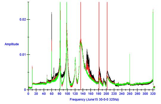
Figure 36: Amplitude vs. Frequency (with
noise)
For purposes of this research the USC-FEA model was helpful an accurate. Eliminate the accelerometer issues and almost half of the problems in interpreting the graphs resonant frequencies are eliminated. The model is a good one and may be more accurate than led to believe by the graphs. If there was a different method of selecting the resonant frequency the results may be even closer to actual test results, although difficult to believe. For all information gathered within this research the resonant frequencies were selected by the highest spikes on the FFT graphs. Some of these spikes were asymmetrical and some may have been broad spikes spanning as many as 40 Hz at the base. This leaves open the possibility of selecting the wrong frequency as the harmonic frequency. A suggestion would be to select the resonant frequency as follows: First find the two points at which there is the following amplitude near the resonant frequency.
![]() Equation
15
Equation
15
Take those two frequencies x1 and x2 and find the median.
![]() Equation
16
Equation
16
This would give resonant frequencies that incorporated error bars relative to the results, whereas past results are given as single points.
The purpose of this research was not to create a USC-FEA model, but since it is here there are several areas that can be improved on or at least understood more. The troubled areas involve the models inability to accurately model intermediate joint structures, successfully run with light and stiff springs in place of the aluminum bulkhead spacers. There is already data from the actual quarter scale tests; all that needs to be done now is to corroborate these additional data points.
The final suggestion for future works validates the USC-FEA beam adaptation tests with quarter scale beam adaptation tests. With the addition of the two bulkheads for the last set of tests the only information for results exists in the form of an FEA model where not all is known. To create the additional pieces to adapt the quarter scale model, incorporate them into the quarter scale model and run the dynamic tests would create the foundation for the possibility of more adaptations of the beams in order to increase the resonant frequency. Such as the redesign of beam three as a stiffer beam since it carries the largest influence on the traveling resonant frequencies.
[1] Cyril, M.H., Shock and Vibration Handbook, McGraw-Hill (1995).
[2] Giurgiutiu, V., EMCH 883: Wave Propagation in Solids, Fall (2004).
[3] Gurgoze, M, Batan, H., On the Effect of an Attached Spring-Mass System on the Frequency Spectrum of a Cantilevered Beam, Journal of Sound and Vibration (1996) 195 (1), pp. 163-168.
[4] Hibbeler, R.C., Mechanics of Materials, 4th edition.(1999), Chapters 6 and 12.
[5] Lagace, P.A., General Dynamic Considerations, Unit 19 (2001) pp. 19.2-19.22
[6] Lagace, P.A., Vibration of Multi Degree-of-Freedom Systems, Unit 22 (2001) pp. 22.2-22.23.
[7] Li, Q.S, Fang, J.Q, Jeary, A.P., Free Vibration Analysis of Multi-Storey Buildings with Narrow Rectangular Plane Configuration, Engineering Structures 21 (1999) pp. 507-518.
[8] Li, Q.S, Fang, J.Q, Jeary, A.P., Free Vibration Analysis of Cantilevered Tall Structures Under Various Axial Loads, Engineering Structures 22 (2000) pp. 524-534.
[9] Murphy, J. F., Transverse Vibration of a Simply Supported Beam with Symmetric Overhang of Arbitrary Length, Vol. 25, No. 5, September 1997, pp. 522-524.
[10] Pai, P.F., Lee, S.Y., Non-Linear Structural Dynamics Characterization Using a Scanning Laser Vibrometer, Journal of Sound and Vibration 264 (2003) pp. 657-687.
[11] Ranson, W., Engr 710: Dynamic Analysis, University of
[12] Sarkar, P.K., Approximate Determination of the Fundamental Frequency of a Cantilevered Beam with Point Masses and Restraining Springs, Journal of Sound and Vibration (1996) 195 (2), pp. 229-240.
[13] Serway, R.A., Beichner, R.J., Physics for Scientists and Engineers, 5th edition (2000) Chapters 1-2.
[14] Simmons, F III, Investigation of the Dynamic Response of a Segmented Cantilever Beam Subjected to Variable Support Stiffness, 2004.
[15] Smith, J.B., The Modal Analysis of a Cantilevered Tri-Sectioned Beam With Various End Stiffness Configurations, 2003.
[16] Smith, S.T., Chetwynd, D.G., Foundations of Ultraprecision Mechanism Design, Breach Science Publishers (1992).
[17] Thomson, W.T., Theory of Vibration with Applications, 2nd edition 1981.
[18] Thomson, W.T., Dahleh, M.D., Theory of Vibration with Applications, 5th edition 1998.
[18] Vibrational Analysis for Beams Chapter 6.
[19] www.GeneralDynamics.com